Computational Performance

Updated April 2025

Recent information about the computational approach and scaling performance of CGYRO [CBB16, CSB+19, SBCB23, SBCW22] is documented here.

Computational Approach

Library overview

CGYRO is written in Fortran, with GPU accelerator optimizations implemented using OpenACC or OpenMP offloading, and communication with GPU-aware MPI. Heavy use of cuFFT/rocFFT is made for the nonlinear term. Analysis tools are based on Python scripts. Exceptional GPU scaling performance on OLCF Summit has been demonstrated through previous ALCC and INCITE Awards over the years 2019-2024. On Summit, the following modules were used: pgi, spectrum-mpi, fftw, netlib-lapack, essl, cuda, python. In early 2023, CGYRO was ported to OLCF Frontier [SBCB23], and capability-scale simulations using more than 20% of the system were carried out in a 2023-2024 INCITE project. Over 87% of CGYRO usage for our 2024 INCITE was capability-scale (over 90% for 2023 INCITE), using at least 2048 nodes (8192 MI250X accelerators) on Frontier. On Frontier, CGYRO uses the HPE Cray Compiling Environment (CCE) Fortran compiler (PrgEnv-cray, cray-mpich), craype-accel-amd-gfx90a (for GPU-aware Cray mpich), cray-python, rocm and AMD hipfort providing Fortran interfaces for calling HIP libraries hipFFT/rocFFT.

Gyrokinetic framework

CGYRO solves the nonlinear, electromagnetic gyrokinetic equations [SH98] for 5D particle distributions \(\Hf(k_x,k_y,\theta;\xi,{\rm v})\), where the subscript \(a\) is the species index, and tildes indicate a Fourier-space quantity. The spatial coordinates are

(2)\[\begin{split}\begin{align} k_x & \rightarrow \text{radial wavenumber} \; , \\ k_y & \rightarrow \text{binormal wavenumber} \; , \\ \theta & \rightarrow \text{field-line coordinate} \end{align}\end{split}\]

where \(k_\perp^2 = k_x^2 + k_y^2\), and the velocity-space coordinates are

\[\begin{split}\xi = \vpar/{\rm v} & \rightarrow \text{pitch angle cosine} \in [-1,1] \; , \\ {\rm v} & \rightarrow \text{speed} \in [0,\infty] \; .\end{split}\]

The use of twisted fieldline coordinates gives radial wavenumbers \(k_x\) that depend on \(\theta\) and \(k_y\) [CBB16]. For this reason, we define a simple radial wavenumber \(\kx\) (the value of \(k_x\) at \(\theta=0\)). The \((k_x,k_y)\) spectral representation facilitates the arbitrary wavelength formulation by diagonalizing the gyroradius operator. The GK equations are written in terms of an EM field potential \(\pf\),

(3)\[ \pf = J_{0}(k_\perp \rho_a) \left( \dphif - \frac{\vpar}{c} \dapf \right) + \frac{m_a {\rm v}_{\perp}^2}{z_{a} e B} \frac{J_{1}(k_\perp \rho_a)}{k_\perp \rho_a} \dbpf \; ,\]

where \(m_a, z_a\) and \(\rho_a\) are the species mass, charge and gyroradius. Above, \((\dphif,\dapf,\dbpf)\) are the electrostatic and transverse/compressional EM potentials, respectively, computed from the gyrokinetic Maxwell equations [SH98]. The Bessel functions \(J_{0}\) and \(J_{1}\) arise from gyroaveraging. In terms of \(\pf\), the GK equation for species \(a\) can be written as

(4)\[\frac{\partial \hf}{\partial \tau} + A(\Hf,\pf) + B(\Hf,\pf) = 0 \; ,\]

with \(\tau \doteq (c_s/a) t\) the normalized time, \(a\) the separatrix minor radius, \(c_s=\sqrt{T_e/m_D}\) the deuteron (mass \(m_D\)) sound speed, and \(T_e\) the electron temperature. \(A(\Hf,\pf)\) and \(B(\Hf,\pf)\) represent the collisionless and collisional terms, respectively. In Eq. (4), \(\Hf\) is the nonadiabatic distribution whereas \(\hf\) is a modified distribution suitable for numerical time-integration. They are related through the field potential by \(\hf = \Hf - (z_a T_e)/T_a \pf\).

(5)\[\begin{split}\left( k_\perp^2 \lambda_D^2 n_e + \sum_a \frac{z_a^2 T_e}{T_a} n_a \right) \dphif & = \sum_a z_a e \int \hskip -3pt \dv f_{0a} J_0(k_\perp \rho_a) \Hf \; , \\ - \frac{2 n_e}{\betae} k_\perp^2 \rho_s^2 \dapf & = \sum_a z_a e \int \hskip -3pt \dv \frac{\vpar}{c_s} f_{0a} J_0(k_\perp \rho_a) \Hf \; \\ -\frac{2 n_e}{\betae} \frac{B}{B_{\rm unit}} \dbpf & = \sum_a \int \hskip -3pt \dv \frac{m_a {\rm v}_{\perp}^2}{T_e} f_{0a} \frac{J_1(k_\perp \rho_a)}{k_\perp \rho_a} \Hf \; .\end{split}\]

Here \(\lambda_D = \sqrt{T_e/(4 \pi n_e e^2)}\) is the Debye length and \(\betae = 8 \pi n_e T_e/\bunit^2\) is the effective electron beta, where \(\bunit\) is the effective magnetic field [CB10].

Time advance

Operator splitting is used to separate the evolution of \(A(\Hf,\pf)\) and \(B(\Hf,\pf)\). This allows the nonlinear, collisionless dynamics \((A)\) to be treated explicitly, while the collisional dynamics \((B)\) is advanced implicitly. First, the collisionless step operates primarily on the spatial dimensions and is distributed in the velocity dimensions, requiring solution of

(6)\[\frac{\partial \hf}{\partial \tau} + A(\Hf,\pf) = 0 \; .\]

We write the collisionless term as:

(7)\[\begin{split}\begin{multline} A(\Hf,\pf) = -i \left( \Omega_{\rm parallel} + \Omega_{\rm drift} \right) \Hf - i \Omega_* \pf -i \Omega_s X \hf \\ \qquad - \frac{c}{B} \frac{a}{c_s} \sum_{\kpv^\prime + \kpv^{\prime \prime} = \kpv} \left( \bhat \cdot \kpv^\prime \times \kpv^{\prime \prime} \right) \pf(\kpv^\prime) \hf(\kpv^{\prime \prime}) \; . \end{multline}\end{split}\]

The linear terms in \(A\) include the parallel streaming along the field line \(\Omega_{\rm parallel}\), drift motion perpendicular to the field line \(\Omega_{\rm drift}\), instability drive from equilibrium density and temperature gradients \(\Omega_*\), and \(\exb\) shear (see Ref. [CBB16]). These linear terms define the streaming kernel, hereafter referred to as str. The last term in Eq. (7) is a convolution (Poisson bracket in real space). This defines the nonlinear kernel and is hereafter referred to as nl. Note that global capability (profile-curvature, or radial profile variation of the plasma density, temperature, and rotation of the equilibrium state) is enabled using a novel wavenumber advection scheme [CB18, CBS20]. Explicit coupling with the Maxwell equations is also required to advance \(\pf\) in time. This operation defines the field solve kernel, hereafter referred to as field. To advance Eq. (6), RK4 or adaptive RK5(4)/RK7(6) methods are used.

The collisional step acts primarily on velocity dimensions and is distributed in the spatial dimensions:

(8)\[\frac{\partial \hf}{\partial \tau} + B(\Hf,\pf) = 0 \quad \text{where} \quad B(\Hf,\pf) = -i \Omega_{\xi} \Hf - \frac{a}{c_s} \sum_b C_{ab}^{L}(\Hf,\Hfb) \; .\]

Here \(-i \Omega_{\xi}\) describes linear trapped particle motion, and \(C_{ab}^{L}\) is the Sugama cross-species collision operator [SWN09], which describes pitch-angle and energy diffusion. This is one of the most sophisticated collision operators available in numerical gyrokinetics. A Legendre pseudospectral discretization in \(\xi\) is combined with a Steen pseudospectral discretization in \({\rm v}\). Using a weak form of the discrete collision matrix, we construct a self-adjoint pseudospectral representation. An implicit time-advance is necessary for stability without severe accuracy loss. Using a generalization of the Crank-Nicolson method, Eq. (8) is advanced with a single matrix-vector multiply (matrix rank \(N_\xi N_v N_a\)). The matrix is large and well-suited to execution on GPUs. The collision kernel is hereafter referred to as coll.

FFT-based evaluation of the nonlinearity

Evaulation of the quadratic nonlinearity in Eq. (7) is done in a standard way using a 2D dealiased FFT [Ors71]. To prevent aliasing, we zero-pad the spectral representation by a factor of \(3/2\). The convolution conserves important flow invariants and eliminates a class of nonlinear instabilities from the numerical solution. To perform the forward and inverse FFTs, we use FFTW [FJ05] by default with options for cuFFT/rocFFT (GPU) on Summit/Frontier and Intel MKL on supported platforms. First, we perform a series of four 2D complex-to-real (c2r) transforms:

\[\begin{split}(i k_x) \pf & \underset{\mathtt{c2r}}{\longrightarrow} \frac{\partial \Psi_a}{\partial x} \, , \\ (i k_x) \hf & \underset{\mathtt{c2r}}{\longrightarrow} \frac{\partial h_a}{\partial x} \, , \\ (i k_y) \pf & \underset{\mathtt{c2r}}{\longrightarrow} \frac{\partial \Psi_a}{\partial y} \, , \\ (i k_y) \hf & \underset{\mathtt{c2r}}{\longrightarrow} \frac{\partial h_a}{\partial y} \; ,\end{split}\]

where \(x\) and \(y\) are real-space meshpoints, such that all arrays are extended and zero-padded by a factor of \(3/2\) (quantities without tildes are in real space). The real-space products are then taken, followed by the inverse transform of the entire nonlinearity via a single 2D real-to-complex r2c transform

\[- \frac{\partial \Psi_a}{\partial x} \frac{\partial h_a}{\partial y} + \frac{\partial h_a}{\partial x} \frac{\partial \Psi_a}{\partial y} \underset{\mathtt{r2c}}{\longrightarrow} \left( \bhat \cdot \kpv^\prime \times \kpv^{\prime \prime} \right) \pf(\kpv^\prime) \hf(\kpv^{\prime \prime}) \; .\]

Table 31 Summary of data properties of kernels. str refers to parallel streaming, field refers to the solution of the three Maxwell equations, coll refers to the implicit collision step, and nl refers to the nonlinear bracket (convolution). In each case, the communication cost associated with each kernel is denoted by the comm suffix.

Kernel	Data dependence	Dominant operation
str	\({\kx,\theta},[k_y]_2,[\xi,{\rm v},a]_1\)	loop
field	Same as str	loop
coll	\([\kx,\theta]_1,[k_y]_2,\xi,{\rm v},a\)	mat-vec multiply
nl	\({\kx,k_y},[\theta,[\xi,{\rm v},a]_1]_2\)	FFT
str_comm	\({\kx,\theta},[k_y]_2,\underline{[\xi,{\rm v},a]_1}\)	MPI_ALLREDUCE
field_comm	Same as str_comm	MPI_ALLREDUCE
coll_comm	\(\kx,\theta,[k_y]_2,[\xi,{\rm v},a]_1\)\(\leftrightarrow [\kx,\theta]_1,[k_y]_2,\xi,{\rm v},a\)	MPI_ALLTOALL
nl_comm	\(\kx,\theta,[k_y]_2,[\xi,{\rm v},a]_1\)\(\leftrightarrow \kx,k_y,[\theta,[\xi,{\rm v},a]_1]_2\)	MPI_ALLTOALL

Array layouts and communication

There are three computational array layouts. Two are associated with the linear terms, and the third with the nonlinear kernel. Internally, we define lumped variables for convenience; the configuration pair \((\kx,\theta)\) uses a single array with length \(\mathtt{nc} = N_x \times N_\theta\), and the velocity triplet \((\xi,{\rm v},a)\) uses a single array with length \(\mathtt{nv} = N_\xi \times N_{\rm v} \times N_a\). In the binormal direction, \(N_y\) values of \(k_y\) are simulated, with the \(h_a\) for different values of \(k_y\) independent in the linear case. First, there is a collisionless layout for the linear terms in \(A(\Hf,\pf)\) with nc configuration space gridpoints on an MPI task, but distributed in velocity space (nv gridpoints) on communicator 1 and in \(k_y\) on communicator 2 (with a single \(k_y\) per task):

\[\mathtt{h(ic,iv\_loc)} \longrightarrow \underbrace{\kx,\theta}_{\mathtt{ic}},[k_y]_2,\underbrace{[\xi,{\rm v},a]_1}_{\mathtt{iv\_loc}} \; .\]

There is no distributed \(k_y\) index because there is one value of \(k_y\) per MPI task. The collisional layout for \(B(H_a,\Psi_a)\) has all of velocity space on an MPI task, but is distributed in configuration space:

\[\mathtt{h(ic\_loc,iv)} \longrightarrow \underbrace{[\kx,\theta]_1}_{\mathtt{ic\_loc}},[k_y]_2,\underbrace{\xi,{\rm v},a}_{\mathtt{iv}} \; .\]

Finally, there is a nonlinear layout

\[\mathtt{h(ir,j\_loc,in)} \longrightarrow \underbrace{\kx}_{\mathtt{ir}},\underbrace{[\theta,[\xi,{\rm v},a]_1]_2}_\mathtt{j\_loc}, \underbrace{k_y}_\mathtt{in} \; .\]

To switch from the collisionless to the collisional layout and back, we use a collision communication (coll_comm). To treat the nonlinearity in \(A(\Hf,\pf)\), the linear process grid is multiplied by \(N_y\) and all toroidal modes are collected on a single core using the nonlinear communication (nl_comm). These two communication operations use MPI_ALLTOALL, but only on a single (not both) MPI subcommunicator. A relatively inexpensive field communication (field_comm) based on MPI_ALLREDUCE solves the Maxwell equations. Finally, there is a communication associated with the conservative upwind scheme (str_comm). The eight computational kernels are summarized in Table 31.

Parallel Performance and Scalability

Strong-scaling performance

Part (a) of Fig. 1 shows strong-scaling results for two CPU-only architectures (NERSC Cori (KNL) and TACC Stampede2 (Skylake)) and three hybrid-CPU/GPU architectures (OLCF Summit, NERSC Perlmutter, and OLCF Frontier). For clarity, we restrict ourselves to simple node-based comparisons. The benchmark test case nl03 is broadly representative of our targeted simulations at coarser resolution, being somewhere between traditional ion-scale resolution and full multiscale resolution with \((N_x,N_y,N_\theta,N_\xi, N_v, N_a) = (512,128,32,24,8,3)\). All systems scale well, with Frontier and Perlmutter by far the best performers on both a per-node and maximum performance basis.

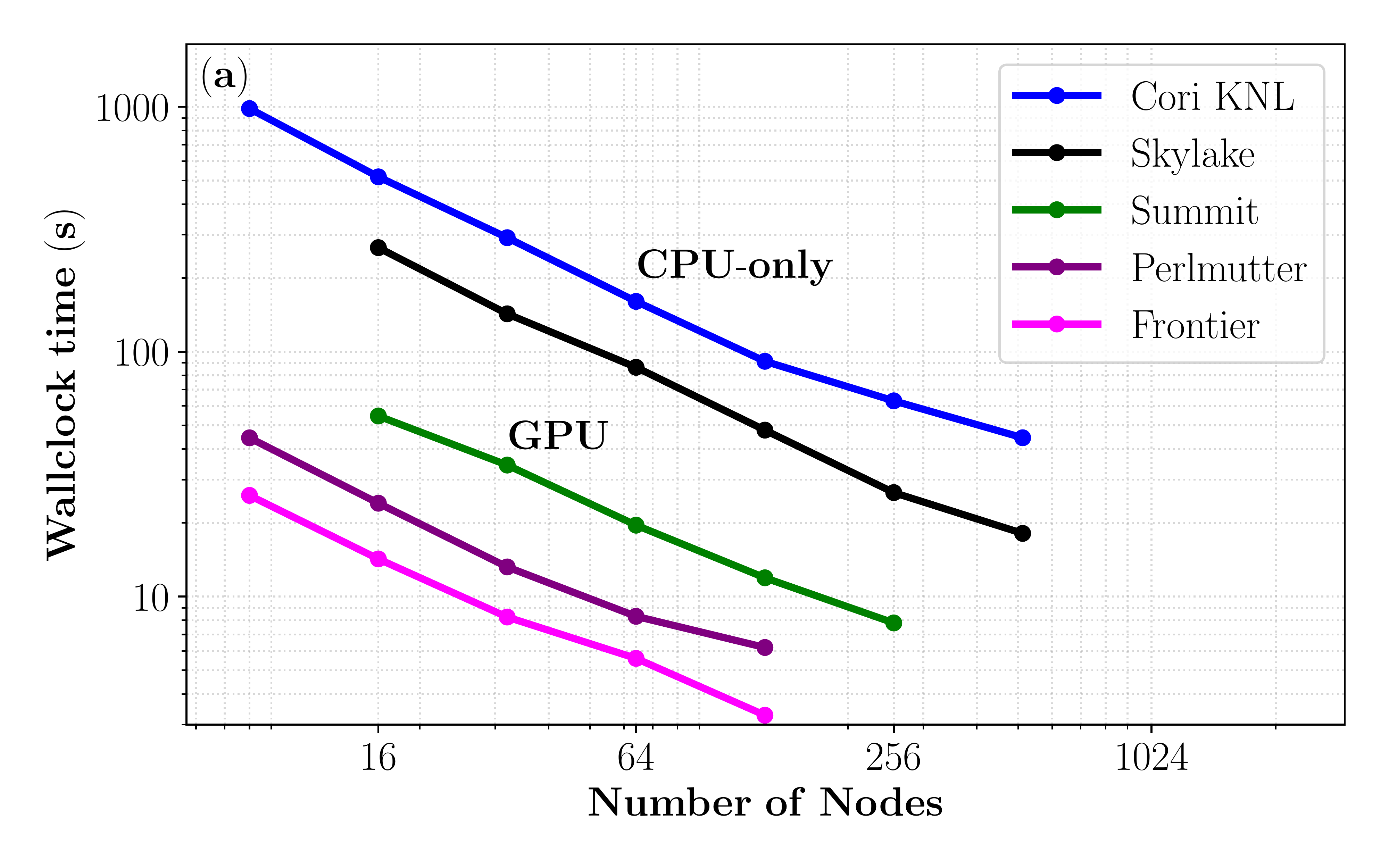
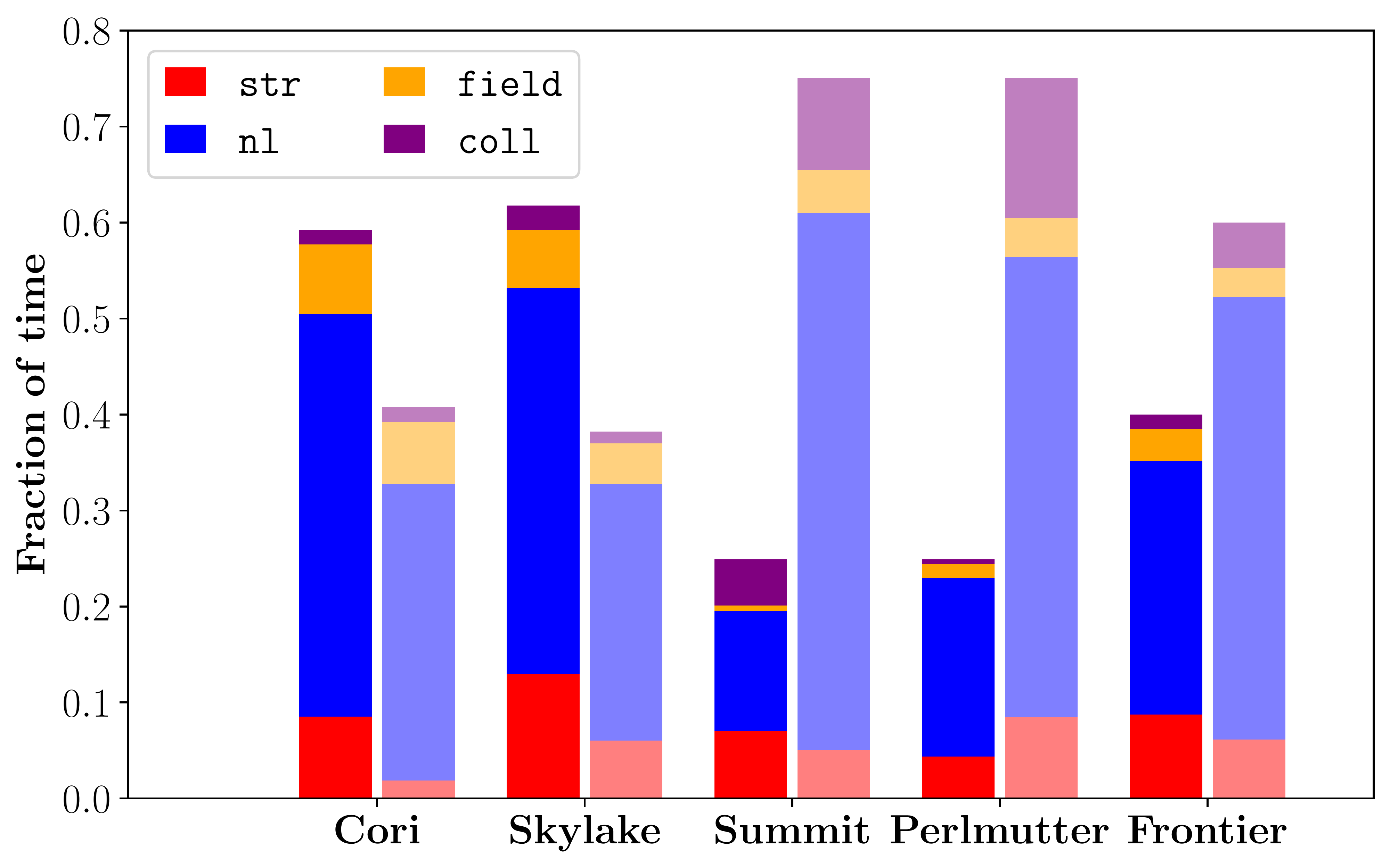
Fig. 1 The (a) Multi-platform strong-scaling comparison for CGYRO test case nl03, showing wallclock time vs. number of nodes. Frontier is by far the best performer on both a per-node and maximum performance basis. (b) Kernel-level analysis. Left (darker) bars indicate compute time; right (faded) bars indicate the communication time. Data is normalized to the total time, such that total bar area is constant (1.0). Lower compute-to-communication ratio on GPU systems reflects the extremely high performance of the GPUs. Note the significant improvement in communication management from Summit/Perlmutter to Frontier.

Kernel-based performance analysis

Part (b) of Fig. 1 shows a breakdown of the time spent in each computational kernel (see Table 31). Data for the CPU-only systems is taken at 128 nodes for Cori and 64 nodes for Skylake. Data for the GPU architectures is taken at 32 nodes. The data is normalized to the total time, ensuring that the total bar area is constant. On the CPU systems, the compute time is dominated by nl. This is a feature of the spectral algorithm that pushes the computational burden to the nonlinear (FFT) term. On the GPU systems, the high performance of cuFFT/rocFFT means a relatively short time spent in nl. This is evident in the small area of the solid blue bar on all GPU systems. On CPU systems, the time spent in nl is higher. A second apparent feature of the kernel timings is the high cost of the nonlinear communication, nl_comm, implemented using MPI_ALLTOALL communication outside the FFT library. On the CPU systems, the cost of nl_comm is always smaller than the cost of nl, whereas on the GPU systems the opposite is true. Importantly, this result is due to extremely high GPU performance, rather than poor interconnect performance. On the GPU systems, CGYRO heavily leverages GPU-aware MPI, giving a 30-40% reduction in communication timing. Fig. 1 part (b) also shows a significant improvement in communication management from Summit/Perlmutter to Frontier, due to optimizations from the porting to Frontier, which are discussed in the next section.

Parallel I/O performance

CGYRO output and checkpointing data are in binary format (single and double precision, respectively). CGYRO I/O implements MPI-IO for parallel/collective-write to single individual files. In our experience, I/O takes less than 2% of total time in production runs on Frontier. We remark that I/O timings for the Orion filesystem on Frontier were found to be nearly twice as fast as Alpine on Crusher/Summit.

Porting and Optimizing for OLCF Frontier

Here we elaborate on the development work that was undertaken in early 2023 for porting and optimizing CGYRO for Frontier. From an application perspective, Frontier’s node architecture is very similar to Summit’s: a multicore CPU is connected by high-speed links to multiple GPUs as accelerators. On Summit, each of the two 21-core IBM P9 CPUs is connected to three Nvidia V100 GPUs by NVLink. On Frontier, one 64-core AMD EPYC 7A53 CPU is connected by AMD Infinity Fabric to four AMD Instinct MI250X accelerators. Each of these accelerators consists of two modules, such that an application sees eight GPUs on a Frontier node. Thus, porting CGYRO from NVIDIA GPU-based systems like Summit and Perlmutter to AMD GPU-based systems like Frontier was relatively straightforward, but performance optimization required more fine-tuning, as described next.

CGYRO uses OpenACC directives to offload computational kernels to GPU accelerators. On Frontier, OpenACC is supported by the HPE Cray Compiling Environment (CCE) Fortran compiler [cce]. Compilation (first on the OLCF testbed system Crusher) was relatively straightforward and required only minimal code changes to CGYRO, mainly related to explicit specification of fields in existing OpenACC directives that were optional for the NVIDIA compiler. For performing FFTs, on Frontier CGYRO calls the hipFFT marshaling library, which in turn uses the optimized rocFFT library for AMD GPUs [hipa, roc]. The hipFFT library provides exactly the same interface as the cuFFT library to ease porting. We also use AMD hipfort, which provides Fortran interfaces for calling HIP libraries [hipb].

In the optimization effort on Frontier, some fine-tuning was needed to improve performance and scalability. Specifically, it was discovered that the CCE compiler was less capable of automatically choosing the ideal parallelization strategy for some loops, compared to the NVIDIA compiler. Thus, explicitly directing the compiler to use the OpenACC gang vector parallelization was needed for optimal performance. This was mainly important for the stream kernel and field kernel. A sequence of optimizations addressing dominant loop operations was also implemented. In the stream kernel, we reordered loops to remove the need for reductions. In the shear kernel, we removed an intermediary table, trading memory intensity for compute intensity. In both cases, the new code was faster on both AMD and NVIDIA GPU-based systems, but the overall impact was significantly larger for the AMD GPUs. Performance gains comparing the original and optimized code are shown in Fig. 2. For the nonlinear kernel (FFT), we also improved the zero-padding scheme used to avoid aliasing to provide decompositions that eliminate large primes. Significant speed-ups were then observed on all platforms, but more so on the AMD GPU-based system (factor of 3 for test cases), indicating that NVIDIA libraries are more tolerant of sub-optimal programming patterns. This is shown in Fig. 3. Taken altogether, CGYRO performance on the AMD GPU-nodes on OLCF Frontier is now faster than on the NVIDIA GPU-based nodes on NERSC Perlmutter, as summarized in Fig. 4. In addition, with these optimizations for Frontier, modest speed improvements were also seen on NVIDIA GPUs, which was an unexpected benefit.

For the communication, CGYRO heavily leverages GPU-aware MPI on Summit to optimize communication performance. On Frontier, GPU-aware MPI – passing GPU memory addresses directly to MPI routines – is not only supported but is also the recommended way to perform MPI communications, since each of the four HPE Slingshot Network Interface Controller (NIC) is directly connected to the four AMD MI250X GPUs. In comparison with Perlmutter, we found that the in-node communication capabilities of Frontier are almost identical. However, we also found that the dedicated NIC-setup in the Frontier system delivers greater performance than the shared-NIC setup in Perlmutter, as shown in Fig.~ref{fig.amd}d.

Below we show CGYRO performance optimizations from porting to Frontier, comparing wallclock benchmark timings (s) of the Frontier AMD GPU-based system with the Perlmutter NVIDIA GPU-based system, both using 24 GPUs. Original indicates before the Frontier-porting effort. Performance on both systems was improved in all cases.

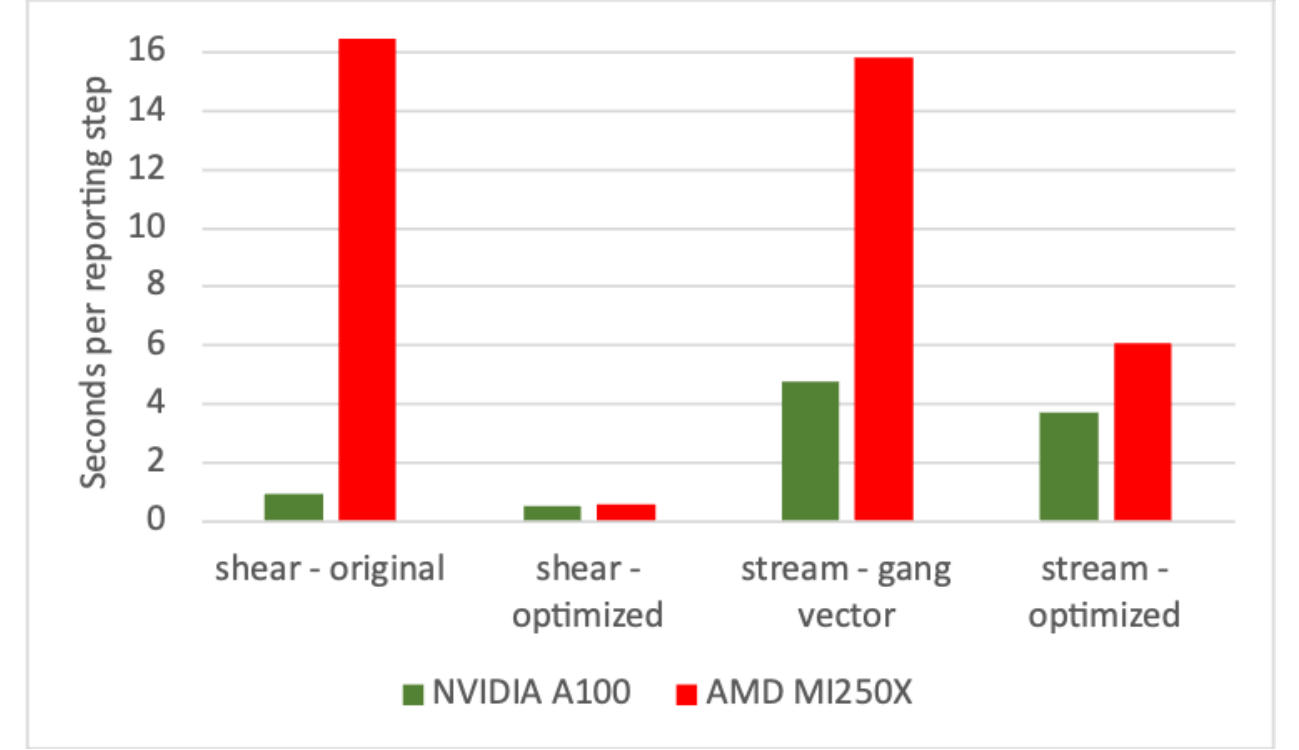
Fig. 2 CGYRO performance optimization results from porting to Frontier, comparing original and optimized shear and stream kernels.

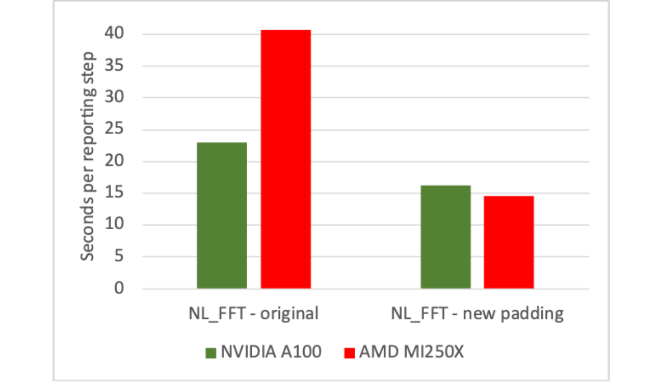
Fig. 3 CGYRO performance optimization results from porting to Frontier, comparing original and optimized nonlinear FFT kernel.

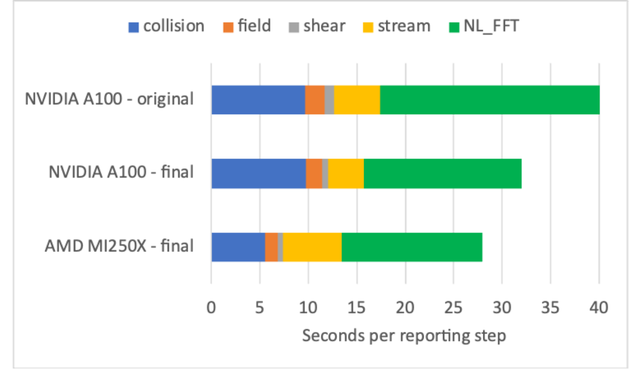
Fig. 4 CGYRO performance optimization results from porting to Frontier, comparing original and optimized overall compute time.

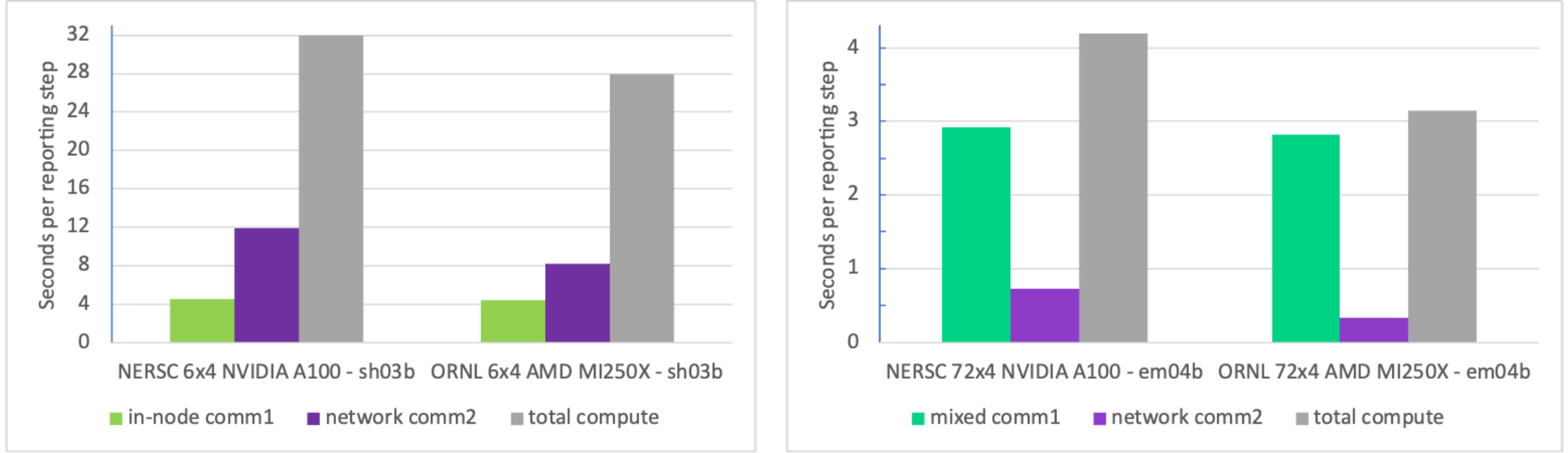
Fig. 5 CGYRO performance optimization results from porting to Frontier, showing communication benchmark with final code.